Integrating Relational Databases with Essbase Studio

Integrating Relational Databases with Essbase Studio

Because relational databases can store several terabytes of data, they offer nearly unlimited scalability. Multidimensional databases, generally smaller than relational databases, offer sophisticated analytic capabilities. By integrating a relational database with an Essbase database, you leverage the scalability of the relational database with the conceptual power of the multidimensional database.

By default, when Essbase Studio creates an Essbase outline, it loads all member levels specified in the metaoutline into a multidimensional database. You can, however, set Essbase Studio to build to a specified member level (Hybrid Analysis) or build only to the dimension level (Advanced Relational Access). Building down to a specified level produces a smaller multidimensional database and a smaller Essbase outline.

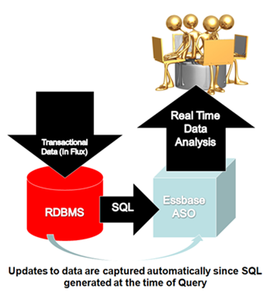
A source relational database can be integrated with an Essbase database by using XOLAP (extended online analytic processing). This is a variation on the role of OLAP in business intelligence. Specifically, XOLAP is an Essbase multidimensional database that stores only the outline metadata and retrieves data from a relational database at query time. XOLAP thus integrates with an Essbase database, leveraging the scalability of the relational database with the more sophisticated analytic capabilities of a multidimensional database.

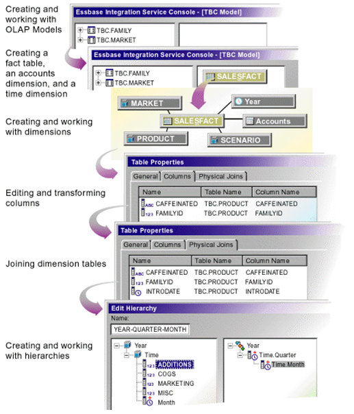
Essbase Studio - Model Development Workflow

Some XOLAP Specifics

• XOLAP (extended online analytic processing) is a variation on the role of OLAP in business intelligence. Specifically, XOLAP is an Essbase multidimensional database that stores only the outline metadata and retrieves data from a relational database at query time. XOLAP thus integrates a source relational database with an Essbase database, leveraging the scalability of the relational database with the more sophisticated analytic capabilities of a multidimensional database.


• OLAP and XOLAP store the metadata outline and the underlying data in different locations:


• 
  
  
  
  • In OLAP, the metadata is located in the Essbase database, and the underlying data is also located in the Essbase database.
  
  
  • In XOLAP, the metadata is located in the Essbase database while the underlying data remains in your source relational database.
  
  
  
  

• The differences in the locations of the metadata and data are key to understanding how XOLAP can be of benefit because these differences affect the functionality of OLAP and XOLAP.


• OLAP lends itself to traditional relational data storage and data analysis. XOLAP lends itself to operations supported in mixed or "hybrid" environments such as Hybrid Analysis and Advanced Relational Access (familiar to users of Essbase and Essbase Studio). Many of the basic concepts of Hybrid Analysis and Advanced Relational Access have been folded into the functionality of XOLAP cubes in Oracle Essbase Studio.

XOLAP Workflow

The workflow of data retrieval in an XOLAP environment is much like that of a non-XOLAP environment:

1. The model is designated as XOLAP-enabled in Essbase Studio.


2. The cube is deployed in Essbase Studio; however, no data is loaded at that time.


3. The Essbase database is queried, using Smart View, Oracle Essbase Visual Explorer, or another reporting tool which can access an Essbase database.


4. Essbase dynamically generates the required SQL to retrieve the data from the source relational database.

Integrating XOLAP with Traditional OLAP Sources

XOLAP has the following restrictions:

1. No editing of an XOLAP cube is allowed. If you wish to modify an outline, you must, instead, create a new outline in Oracle Essbase Studio. XOLAP operations will not automatically incorporate any changes in the structures and the contents of the dimension tables after an outline is created.


2. When derived text measures are used in cube schemas to build an Essbase model, XOLAP is not available for the model.


3. XOLAP can be used only with Aggregate Storage. The database is automatically duplicate-member enabled.


4. XOLAP supports dimensions that do not have a corresponding schema-mapping in the catalog; however, in such dimensions, only one member can be a stored member.

Usages Not Supported in XOLAP

XOLAP does not support use of the following:

• Flat files


• Ragged hierarchies


• Alternate hierarchies


• Recursive hierarchies


• Calendar hierarchies


• Filters


• Typed measures


• User defined members at the leaf level


• Multiple relational data sources

Hybrid Analysis

Hybrid Analysis eliminates the need to load and store lower-level members and their data within the Essbase database. This feature gives Essbase the ability to operate with almost no practical limitation on outline size and provides for rapid transfer of data between Essbase databases and relational databases.


Hybrid Analysis integrates a relational database with an Essbase multidimensional database so that applications and reporting tools can retrieve data directly from both databases.

Data Flow for Hybrid Analysis

• The initial step in setting up XOLAP or Hybrid Analysis is to define the relational database as a XOLAP or Hybrid Analysis relational source.

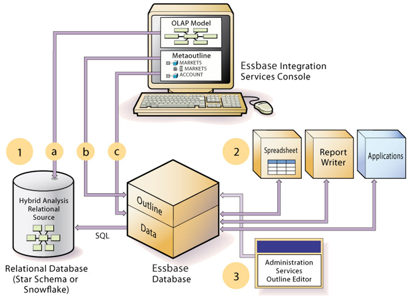
1. You define the XOLAP or Hybrid Analysis relational source in Essbase Studio. Through Essbase Studio, you first specify the relational data source for the OLAP model. The OLAP model is a schema that you create from tables and columns in the relational database. To build the model, Essbase Studio accesses the star schema of the relational database. Using the model, you define hierarchies and tag levels whose members are to be enabled for Hybrid Analysis. You then build the metaoutline, a template containing the structure and rules for creating the Essbase outline, down to the desired Hybrid Analysis level. The information enabling Hybrid Analysis is stored in the OLAP Metadata Catalog, which describes the nature, source, location, and type of data in the Hybrid Analysis relational source.


2. Next, you perform a member load, which adds dimensions and members to the Essbase outline. At this point XOLAP databases are complete and can queried by a multitude of reporting tolls.


3. For Hybrid Analysis databases, when the member load is complete, you must run a data load to populate the Essbase database with data.

• Applications and reporting tools, such as spreadsheets and Report Writer interfaces, can retrieve data directly from both databases using the dimension and member structure defined in the outline, Essbase determines the location of a member and then retrieves data from either the Essbase database or the Hybrid Analysis relational source if a Hybrid Analysis database and from the relational data source when a XOLAP model is specified.
  
  
  
  
  
  • If the data resides in the Hybrid Analysis relational source, Essbase retrieves it through SQL commands.
  
  
  • XOLAP also leverages transactional SQL to access data from the fact table at the time the query is initiated by the end user.
    
    
  
  
  
  


• To modify the outline in Hybrid Analysis, you can use Outline Editor in Administration Services to enable or disable dimensions for Hybrid Analysis on an as-needed basis. Changes to metadata in XOLAP require a complete drop and rebuild of the Application and database through Essbase Studio

Comparison of Aggregate and Block Storage

Since XOLAP only supports the Aggregate Storage Kernel, it is pertinent to highlight the differences in ASO and BSO.

Essbase provides an aggregate storage kernel as a persistence mechanism for multidimensional databases. Aggregate storage databases enable dramatic improvements in both database aggregation time and dimensional scalability. The aggregate storage (ASO) kernel is an alternative to the block storage (BSO) kernel. Aggregate storage databases typically address read-only, "rack and stack" applications that have large dimensionality, such as the following applications:

• Customer analysis. Data is analyzed from any dimension, and there are potentially millions of customers.


• Procurement analysis. Many products are tracked across many vendors.


• Logistics analysis. Near real-time updates of product shipments are provided.

Aggregate storage applications, which differ from block storage applications in concept and design, have limitations that do not apply to block storage applications.

Inherent Differences between ASO and BSO

Inherent Differences	Aggregate Storage	Block Storage
Storage Kernel	Architecture that supports rapid aggregation, optimized to support high dimensionality and sparse data	Multiple blocks defined by dense and sparse dimensions and their members, optimized for financial applications
Physical Data Storage	Through the Application Properties window, Tablespaces tab in Administration Services	Through the Database Properties window, Storage tab in Administration Services
Databases supported per application	One	Several (one recommended)

Outline Differences with ASO and BSO

Outline Functionality	Aggregate Storage	Block Storage
Multiple hierarchies enabled, dynamic hierarchy, or stored hierarchy designation	Relevant	Irrelevant
Accounts dimensions and members on dynamic hierarchies	Support with the following exceptions: • No two-pass calculation • No association of attribute dimensions with the dimension tagged Accounts • Additional restrictions for shared members.	Full support
Members on stored hierarchies	Support with the following exceptions: • Support for the ~ (no consolidation) operator (underneath label-only members only) and the + (addition) operator • Cannot have formulas • Restrictions on label only members • No Dynamic Time Series members • Stored hierarchy dimensions cannot have shared members. Stored hierarchies within a multiple hierarchies dimension can have shared members.	Full support
Member storage types	Support with the following exceptions: • Dynamic Calc and Store not relevant • On stored hierarchies, two limitations if a member is label only: o All dimension members at the same level as the member must be label only o The parents of the member must be label only.	Support for all member storage types in all types of dimensions except attribute dimensions

Calculation Differences between ASO and BSO

Calculation Functionality	Aggregate Storage	Block Storage
Database calculation	Aggregation of the database, which can be predefined by defining aggregate views	Calculation script or outline consolidation
Formulas	Allowed with the following restrictions: Must be valid numeric value expressions written in MDX No support for Essbase calculation functions On dynamic hierarchy members, formulas are allowed without further restrictions	Support for Essbase calculation functions
Calculation scripts	Not supported	Supported
Attribute calculations dimension	Support for Sum	Support for Sum, Count, Min, Max, and Average
Calculation order	Member formula calculation order can be defined by the user using the solve order member property	Defined by the user in the outline consolidation order or in a calculation script

Partitioning Differences between ASO and BSO

Partitioning Functionality	Aggregate Storage	Block Storage
Partitioning	Supported with the following restrictions: No Outline Synchronization	Fully supported

Data Load Differences between ASO and BSO

Data Load Functionality	Aggregate Storage	Block Storage
Cells loaded through data loads	Only level 0 cells whose values do not depend on formulas in the outline are loaded	Cells at all levels can be loaded (except Dynamic Calc members)
Update of database values	At the end of a data load, if an aggregation exists, the values in the aggregation are recalculated	No automatic update of values. To update data values, you must execute all necessary calculation scripts.
Data load buffers	The loading of multiple data sources into aggregate storage databases is managed through temporary data load buffers.	Not supported
Atomic replacement of the contents of a database	When loading data into an aggregate storage database, you can replace the contents of the database or the contents of all incremental data slices in the database.	Not supported
Data slices	Aggregate storage databases can contain multiple slices of data. Data slices can be merged.	Not supported
Dimension build for shared members	Full support for parent-child build method. Duplicate generation (DUPGEN) build method limited to building alternate hierarchies up to generation 2 (DUPGEN2).	Support for all build methods
Loading data mapped to dates	In a date-time dimension, you can load data into level-0 members using supported date-format strings instead of member names.	Date-time dimension type is not supported.

Query Differences between ASO and BSO

Query Functionality	Aggregate Storage	Block Storage
Report Writer	Supported, except for commands related to sparsity and density of data	Fully supported
Spreadsheet Add-in	Supported, with limited ability to change data (write-back)	Fully supported
API	Supported	Supported
Export	Support with the following restrictions: • Export of level 0 data only (no upper-level export) • No columnar export	Supported
MDX queries	Supported	Supported
Queries on attribute members that are associated with non-level 0 members	Returns values for descendants of the non-level 0 member.	Returns missing for descendants of the non-level 0 member
Queries on attribute members and shared members	A shared member automatically shares the attribute associations of its nonshared member	A shared member does not share the attribute associations of its nonshared member
Query logging	Not Supported	Supported
Query performance	Considerations when querying data from a dimension that has multiple hierarchies.	Hierarchies not relevant

Feature Differences between ASO and BSO

Featues	Aggregate Storage	Block Storage
Aliases	Supported	Supported
Currency Conversion	Not Supported	Supported
Data Mining	Not Supported	Supported
Hybrid Analysis	Support with the following restriction: queries that contain a relational member and an Essbase member with a formula in the same query are not supported.	Supported
Incremental Data Load	Supported	Supported
LROs	Not Supported	Supported
Time Balance Reporting	Support with the following restrictions: • Skip Zeros is not supported • Time dimension must contain at least one stored hierarchy • Shared members must be at level zero	Supported
Triggers	After-update triggers supported	On-update triggers and after-update triggers supported
Unicode	Supported	Supported
Variance Reporting	Not Supported	Supported
Date-time dimension type and linked attribute dimensions	Supported	Not Supported
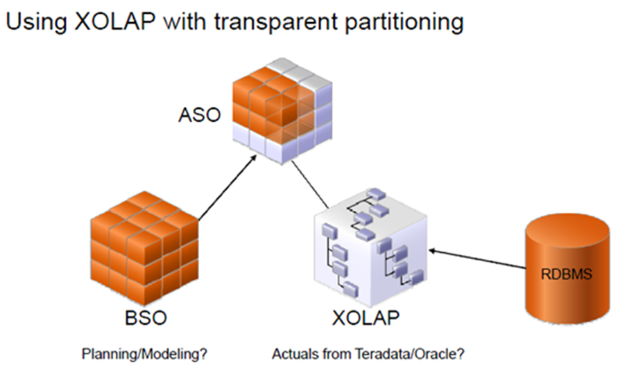
User ability to change data (write-back)	Transparent partition technique used to enable limited write-back	Fully Supported

Links to Blogs written by BICG on XOLAP

Part 1 of the XOLAP blog


http://oraclebiblog.blogspot.com/2010/02/xolap-virtual-cubes-against-data.html

Part 2 of the XOLAP blog


http://oraclebiblog.blogspot.com/2010/02/xolap-virtual-cubes-against-data_15.html

Vintages - Time x Time

One of the more unique conceptual challenges when designing an Essbase or Planning model can revolve around handling multiple Time-basis dimensions. Many model requirements need granularity beyond the standard observation date that is typically defined as being the Time Period in a model. Consider the following:
A customer has a portfolio of investments, each having several characteristics related to some measurement of time.

• The origination date of the investment
• The maturity date of the investment
• An expected length of the investment, based from which the origination or maturation date can be interpreted
• An activity date

A single Time dimension (or two time dimensions that split portions of time apart, i.e. separating Years from Months and Quarters) can not accurately capture metrics in the previous example like the performance over time of all investments that originated in a given period, or how much return at a certain age of an investment can be expected.

Multiple Time Dimensions
Assuming the standard Essbase or Planning time dimensions represent the observation date, additional time-style dimensions can be created to provide more granularity. In the previous example, a dimension indicating the age of an investment can be utilized to analyse performance of investments based on how long ago they were originated. Likewise, identification of the starting or ending dates of investments allows analysis based on similar origination or maturation dates.

How much is too much granularity?
That all depends on the analysis requirements for a model. Adding more detail to a model will increase its size and complexity, but will provide a more detailed picture of time's effect on activity. All decisions regarding expanding a model require careful considerations of the benefits of additional complexity.



Other Time Time appears multiple Times (Time beyond core modelling requirements)

• Scenario revisions

First pass, second pass, etc: These are essentially observations or snapshots of a process at a point in time. Depending on how many of these snapshots are required, it may be advantageous to have a separate dimension identifying when the snapshot was presented. Consider the benefits carefully of disposing of forecast revisions. Often, one key long term goal to improve forecast reliability is the ability to track variances between revisions over time.

Attributes, UDAs, and Alternate Hierarchies

I'm often asked what the best practice is regarding implementation of Attribute Dimensions, Alternate Hierarchies, and User Defined Attributes. While there are no hard and fast rules, these guidelines outline the strengths and weaknesses of each.

Attribute Dimensions
Attribute dimensions are created by tagging members in a sparse dimension with an attribute tag. Members tagged with a member from an attribute dimension must be at the same Level as all other members tagged with an attribute from the respective attribute dimension. In theory, as long as members are at the same level they may be assigned attributes. In practice I recommend avoiding utilizing attributes for members that are not level zero members. This is due to difficulties ensuring members are at the same level. While this often is apparent in ragged hierarchies (also known as unbalanced hierarchies), symmetrical hierarchies can also have members that appear to be at the same level (i.e. they are at the same generation), but are in fact at different levels due to implied sharing where a parent only has one child. Also, this can create situations where a member is at multiple levels, and the resulting data value utilized by an attribute is not what a user expects.

User Defined Attributes (UDAs)
UDAs are flags that are placed on an Essbase member. A given UDA can be placed on any dense or sparse member in the outline. In addition, unlike Attribute dimensions, UDAs are not linked to the level of the members they are tagged to. In practice, this flexibility is most often leveraged to identify member sets for use in a calculation, especially since UDAs can be tagged to Dense members. While it is possible to refer to UDAs in most reporting and analysis packages, however, I do not recommend deploying UDAs for use by end users.

Alternate Hierarchies
Alternate hierarchies are secondary rollups of members within the same dimension. The level zero members in the alternate hierarchy are called Shared Members, and point back to an identically named real member elsewhere in the dimension. It is important to note that the real members do not have to be level zero members, or at the same level. One of the key advantages of Alternate Hierarchies is the ability for upper level summary members to have a completely unique structure (as opposed to utilizing an Attribute dimension, which merely re-totals the same hierarchy with only a subset of members). While there are many uses for this functionality, this often is utilized to build Management and Legal organizational hierarchies from the same source data, as well as facilitate financial reporting with different standards (i.e. IFRS vs. US GAAP). Conversely, Alternate Hierarchies typically require more maintenance, and increase the size of database. Therefore, they should be carefully deployed only in circumstances that justify the additional expense.


In summary, Attribute Dimensions, User Defined Attributes, and Alternate Hierarchies all have advantages and disadvantages. A typical deployment will often leverage all three areas of functionality to solve specific business problems, but will pay particular attention to the negatives of each option to prevent creating an overly difficult to support and expensive database.

Essbase member name manipulation - Net Transshipments

Transshipments
In some Essbase models there is a need to capture two essentially identical elements in separate dimensions. One common example of this is a transshipment model, where it is necessary to identify both the origination and destination of a shipment.

Two Dimensions
The most straightforward, and often user-friendly, manner to accomplish this type of tracking is to have the same hierarchy in two dimensions, with each member prefixed differently (i.e. the Source location members might be prefixed with "TO:" while the Destination members would be prefixed with "FROM:").

Net Shipments
A simple metric to consider in this type of model is often Net Shipments. In a multidimensional database, to calculate Net Shipments, shipments out of a location needs to be subtracted from shipments in (or vice-versa, depending on your preference). Assuming this is being calculated for Location A, the formula might look like:
Shipments -> TO:A -> Total Sources - Shipments -> From:A -> Total Destinations
(I.E. take all of the shipments that are sent to "A", regardless of where they are from, and subtract all of the shipments from "A" regardless of where they go to).

The Problem
The formula is simple and straightforward for one location, and remains similar for all other locations, but, every time a location is added, renamed, or deleted the calculation must be updated manually.

The Solution
Assuming the hierarchies are carefully constructed to always require "TO:" before the source location and "FROM:" before the destination location, Essbase can programatically determine the corresponding member by removing and replacing the prefix.

Components
Several string manipulation functions are required:

• @NAME or @ALIAS: Used to pass either an Essbase Member Name or the respective member's Alias Name to another function as a string.
• @SUBSTRING: This function will return a portion of a string passed to it.
• @CONCATENATE: Used to join two strings together.
• @MEMBER: Turns a string into a reference to a member name.

For this example, I'll also utilize @CURRMBR. This function returns the current member being calculated from a given dimension.

So, to determine the corresponding destination from a member in the source dimension:

1. Turn the current member in the source dimension into a string: @NAME(@CURRMBR("Source"))
2. Remove the prefix "TO:" from the string: @SUBSTRING(@NAME(@CURRMBR("Source")),3)
3. Prefix the new string with "FROM:": @CONCATENATE("FROM:",@SUBSTRING(@NAME(@CURRMBR("Source")),3))
4. Convert the string into a reference to a member: @MEMBER(@CONCATENATE("FROM:",@SUBSTRING(@NAME(@CURRMBR("Source")),3)))

Using this formula, you can fix on the portion of a hierarchy in the Source dimension, and have access to each member's corresponding Destination member. The original example of calculating Net Shipments might look like:
Fix(@RELATIVE("Source",0))
"Net Shipments"(
"Shipments"->"Total Destination" - "Shipments"->"Total Source"->@MEMBER(@CONCATENATE("FROM:",@SUBSTRING(@NAME(@CURRMBR("Source")),3)));
);
ENDFIX

XOLAP - Virtual cubes against a Data Warehouse Part 2

As mentioned in my previous blog, "XOLAP - Virtual Cubes Against a Data Warehouse Part 1", I'll address the following in this installment:

• Completing the Time Hierarchy
  
• Developing the rest of the standard dimensions
  
• Developing a measures dimension
  
• Creating the cube schema
  
• Deploying the cube
  
• Querying the data
  
• Showing real time data updates with XOLAP

When we previously left off we had just finished creating new meta data elements within DimTime. The representation of the "Total Time" hierarchy is exhibited below. Create this hierarchy leveraging the steps used to create the "Total Sales Territory" in Part 1.

Leveraging the hierarchy depicted below, create the "Total Currency" hierarchy


Leveraging the hierarchy depicted below, create the "Measures" hierarchy

Leveraging the hierarchy depicted below, create the "Total Customer" hierarchy

To create the "Total Product" hierarchy, a meta data element, "EnglishProductSubcategoryName" needs to be copied from the DimProductSubCategory table to the DimProduct table.

This can be simply accomplished by right clicking on "EnglishProductSubcategoryName" element within the Metadata Navigator window within Essbase Studio and selecting "Copy".

Pasting this element is as equally simple, highlight the DimProduct table, right click and select Paste.

You are now ready to create the "Total Product" hierarchy as shown below.

Create the "Total Promotion" hierarchy as shown below

You are now ready to create the cube schema.

Access the "Cube Schema Wizard" hotlink from the Essbase Studio "Welcome Page."

The "Cube Schema Wizard" should be displayed as shown below.

Within the "Choose Measures and Hierarchies" dialog window specify a name for the cube schema and then select each of the newly created hierarchies from the left panel and move them to the appropriate panel on the right hand side.

After clicking "Next", the "Cube Schema Options" dialog box should be displayed.

Toggle on the "Create Essbase Model" radial button and provide a name for the model.

In this case I have named my model "XOLAP Adventure WorksModel."

After clicking "Next" the Cube Schema Model should be displayed as depicted below

You are now ready to deploy the cube to Essbase.

Access the "Cube Deployment Wizard" hotlink from the Essbase Studio "Welcome Page."

The "Essbase Server Information" dialog box should now be displayed.

Leverage the previously created withing Part 1 of this blog and select this connection name within the Essbase Server Connection drop down box.

Now specify and Essbase Application Name and Database name. These names are restricted to 8 characters and can not be currently used within your Essbase environment.

Ensure that only the "Build Outline" radial box is the only box toggled on at this point and then select the "Model Properties" button from the lower left of the dialog box.

The "View, edit, and save properties" should now be displayed.

With the "XOLAP Adventure WorksModel" highlighted, select the "General" tab and activate the "XOLAP Model" radial button.

With "Total Time" highlighted, select the "Info" tab and set the dimension type to "Time" and dimension storage to "Dense"

With "Measures" highlighted within the "Info" tab, ensures that measures is set to a dimension type to "Accounts" and dimension storage to "Dense"

Select "Close" and then "Finish"

The following image will be displayed while the cube is being deployed

When successfully completed, a notification of successful deployment will be presented.

Navigate to Oracle Essbase Administration Services and review the application and database just created. Your application should look much the image below:

Remember at this point, the outline is the only thing that has been built, no data has been loaded to the application, nor has an calculation been executed.

Leveraging the Hyperion Add-in, connect to the XOLAP database that you have just created, notice data is present and aggregated. Format your query as exhibited, focusing on the following members:

• Customer:Yang, Jon V
• Measure: Unit Price
• Sales Territory: Australia
• Time: Total Time
• Promotion: No Discount
• Currency: Australian Dollar
• Measures: Fenders, Helmets, Jerseys, Mountain Bikes, Tires and Tubes, Touring Bikes

Notice the Unit Price for the data intersection of Mountain Bikes (3399.99)

Now access the underlying relational database, I have leveraged Microsoft SQL Server Management Studio in this instance.

Open the table FactInternetSales and go to row 88, it should agree with the information depicted in the exhibit below:

Update the Unit Cost for row 88 from 3399.9900 to 999999.99 and commit this value to the database

Execute a retrieve against the spreadsheet set up just moments ago.

Notice the data has changed in the underlying relational repository and also through your ad hoc query tool.

While some restrictions do exist in structuring a XOLAP model, which were mentioned in Part 1 of this blog, the robustness of delivering an application of this nature is pretty self evident.
When asked previously by customers, "Can I do ad hoc, real time analysis against transactional data in my data warehouse?" I often struggled to provide an answer that really meet each of those criteria. Now with XOLAP a definitive approach can certainly be presented to the customer.

XOLAP - Virtual cubes against a Data Warehouse Part 1

Can it be true? Real time ad hoc analysis against a Data Warehouse using an Essbase cube that contains no data?

Well with XOLAP, these capabilities a being brought together. I have created a brief tutorial within this article to demonstrate to overall concept relating to XOLAP.

In Part 1 of this article, I'll discuss:

• Setup that needs to occur to emulate sample
  
• Background into XOLAP
  
• Current restrictions relating to XOLAP
  
• Creating Data Sources in Essbase Studio
  
• Defining a MiniSchema
  
• Defining Standard Hierarchies

Due to the number of screen shots and the size of this blog article, I have set the image properties to small. While the screens may be difficult to decipher within the article, each can be clicked on to be rendered in a much larger resolution for viewing.

Setup The Needs to Occur to Emulate Sample

The example delivered in this article involves leveraging AdventureWorksBI.msi on SQL Server 2005 as the Data Warehouse. This database can be downloaded from http://msftdbprodsamples.codeplex.com/releases/view/4004 . The installer for this download requires you to manually attach the database after installation.

Within the dbo.DimCustomer table add a new column called "ProperName" with a property of "nvarchar(100)."

Update the ProperName column within dbo.DimCustomer using a SQL statement similar to the following :

Update dbo.DimCustomer
Set ProperName = LastName + ', ' + FirstName + ' ' + MiddleName

Within the dbo.DimTime table add 3 new columns called "Month", "Day" and "Year" with each having a property of "nchar(10)."

Update the newly added columns within dbo.DimCustomer using a SQL statement similar to the following :

Update dbo.DimTime
Set Month = DatePart(Month,FullDateAlternateKey)
Set Day = DatePart(Day,FullDateAlternateKey)
Set Year = DatePart(Year,FullDateAlternateKey)

A little background into XOLAP

XOLAP (extended online analytic processing) is a variation on the role of OLAP in business intelligence. Specifically, XOLAP is an Essbase multidimensional database that stores only the outline metadata and retrieves data from a relational database at query time. XOLAP thus integrates a source relational database with an Essbase database, leveraging the scalability of the relational database with the more sophisticated analytic capabilities of a multidimensional database.

OLAP and XOLAP store the metadata outline and the underlying data in different locations:

In OLAP, the metadata and the underlying data are located in the Essbase database.

In XOLAP, the metadata is located in the Essbase database and the underlying data remains in your source relational database.

Restrictions For XOLAP

• No editing of an XOLAP cube is allowed. To modify an outline, you must create a new outline in Essbase Studio. XOLAP operations will not automatically incorporate changes in the structures and the contents of the dimension tables after an outline is created.
  
• When derived text measures are used in cube schemas to build an Essbase model, XOLAP is not available for the model.
  
• XOLAP can be used only with aggregate storage. The database is automatically duplicate-member enabled.
  
• Alternate hierarchies and attribute dimensions are supported; however, attribute hierarchies are not supported.
  
• XOLAP supports dimensions that do not have a corresponding schema-mapping in the catalog; however, in such dimensions, only one member can be a stored member.
  
• A model that is designated as XOLAP-enabled must be deployed to a new Essbase database because incremental builds for XOLAP are not supported.
  

Creating a Data Source

• From the "Essbase Studio - Getting Started" page within Essbase Studio, select the hot link "Data Source Wizard", the "Define Connection" portion of the Connection Wizard is displayed.

• Enter a Connection Name.
  
• Enter an optional Description.
  
• Select the appropriate Data Source Type. For example, if you are creating a connection to a Microsoft SQL Server data source, select Microsoft SQL Server from the drop-down list.
  
• In Server Name, enter the name of server where the database resides.
  
• To use a port number other than the default, clear the Default check box next to Port and enter the correct port number in the text box.If you are using the default port number, you can skip this step.
  
• Enter the User Name and Password for this database.
  
• In Database Name, select "AdventureWorksDB"
  
• Click Test Connection. If the information you entered in the wizard is correct, a message confirms a successful connection.If you entered incorrect information in the wizard, a message is displayed explaining that invalid credentials have been provided. Correct the errors and retest until the connection is successful.
  
• Clicking Next takes you to the Select Tables page of the wizard

Select the following tables for the Select Tables dialog box and then select "Next":

• dbo.DimCurrency
• dbo.DimCustomer
• dbo.DimProduct
• dbo.DimProductSubCategory
• dbo.DimPromotion
• dbo.DimSalesTerritory
• dbo.DimTime
• dbo.FactInternetSales
  
  

The Select MiniSchema dialog is now presented.

• Select the radial button for "Create a new schema diagram"
• Enter a name for this schema, In this instance I used "XOLAP Adventure Works DWSchema"
• Leave "Skip Schema" and "Use Introspection to Detect Hierarchies" unchecked
• Select Next
  
  
• The "Populate Schema" dilog box is displayed. Each of the tables that were previosly selected should be displayed on the right hand panel.
• Select "Next"
  
  
• The "Create Metadata Element" dialog box should now be displayed.
• Toggle on the radial button next to the "XOLAP Adventure Works DW", this should toggle on all members displayed in this dialog window
• Select "Next"
  
  
• The "XOLAP Adventure Works DWSchema" should now be displayed.
  
  
• Navigate back to the "Welcome" screen
• Highlight the "DimSalesTerritory" within the Metadata Navigator. Once highlighted, select the "Hierarchies" hotlink from the "Welcome" screen.
  
  
• Above is a representation of the contents from the DimSalesTerritory table. This is provided to deliver an understanding of how the hierarchy will be developed from the underlying relational table
  
  
• The hierarchy wizard should now be displayed at this point.
• Specify the "Dimension Head Name", in this case "Total Sales Territory" and then drag the "SalesTerritoryGroup" data element from the Metadata Navigator into the Data grid.
• The grid should should now contain the "SalesTerritoryGroup" element. Highlight this element and click "Add" and select "Child"
  
  
• Within the "Select Entity" dialog box, select "SalesTerritoryCountry" and then "OK"
  
  
• Leveraging the same approach for you used for adding "SalesTerritoryCountry", now add "SalesTerritoryRegion" to deliver a hierarchy as depicted above.
  
  
• By right clicking on the "Total Sales Territory" hierarchy data element in the MetaData Navigator panel and selecting "Preview Hierarchy" the above sampling of data should be displayed
  
  
• 
  
  Next, we will create the Time hierarchy for the model. This step will be slightly different, we will leverage the newly create columns in SQL server to build out a time hierarchy.
• With the DimTime metadata element highlighted in the MetaData Navigator, right click and select "New" and "Dimension Element"
  
  
  
  
• The "Edit Properties" dialog window for the new data element should appear.
• Enter "Month Day Year" in the name window
• Paste the following syntax into the Caption Binding window:
• 'trim'( connection : \'XOLAP Adventure Works DW'::'AdventureWorksDW.dbo.DimTime'.'Month' ) "/" 'trim'( connection : \'XOLAP Adventure Works DW'::'AdventureWorksDW.dbo.DimTime'.'Day' ) "/" 'trim'( connection : \'XOLAP Adventure Works DW'::'AdventureWorksDW.dbo.DimTime'.'Year' )
  
  
• Repeat the following steps for "Month Year" and place the following syntax in the caption binding window for "Month Year":
• trim'( connection : \'XOLAP Adventure Works DW'::'AdventureWorksDW.dbo.DimTime'.'Month' ) "/" 'trim'( connection : \'XOLAP Adventure Works DW'::'AdventureWorksDW.dbo.DimTime'.'Year' )
  
  
• Repeat the following steps for "Year" and place the following syntax in the caption binding window for "Year":
• 'trim'( connection : \'XOLAP Adventure Works DW'::'AdventureWorksDW.dbo.DimTime'.'Year' )
  

In my next blog, which should be published shortly I'll address the following:

• Completing the Time Hierarchy
• Developing the rest of the standard dimensions
• Developing a measures dimension
• Creating the cube schema
• Deploying the cube
• Querying the data
• Showing real time data updates
  

Hierarchical Metadata Relationships in Essbase – Pro’s and Con’s

A question that often has to be considered during design of an Essbase database is to establish a relationship between metadata points that could possibility be two separate dimensions. For instance, combining Entity and Project into a single entity dimension with Projects rolling into the entities that are responsible for managing those Projects. The first litmus test that needs to be passed is whether your project has a direct correlation to a specific entity. Essentially, does a one for one relationship exist? Can the Project only be managed by one Entity?

In instances where a Project may roll to many different Entities the debate as to whether combining the dimensions is often eliminated since the size of the dimension could eventually become very large due the numbers of combinations of metadata points that would need to be supported. In earlier versions, member uniqueness would be a constraining factor, that at that time, could only be addressed through member concatenation. Duplicate member names capabilities have since eliminated that constraint.

If the project is only managed by a single entity then Pro's and Con's need to be evaluated.

The Single Dimension Approach

• Con's relating to a Single Entity dimension:
  
  • What-if Modeling would need to be a function of an administrator since they would need to stage the alternate roll-up based upon end-user feedback
    
• Pro's with a Single Entity dimension:
  
  • Relationships between contracts and divisions could be clearly understood by viewing the hierarchical structure
    
  • No need to copy, clear, input or move data by end-users when What-If modeling is being performed since organizational changes could be modeled via alternate hierarchies, leveraging shared members.
    
  • Sparseness of the database is reduced allowing for better performance
    
  • One less dimension for users to have to navigate, reducing the possibility of user getting lost in their data
    
  • One less dimension is necessary to aggregate enhancing application performance and promoting a more dynamic application
    
  • Easier administration of security
    

The Separate Dimension Approach

• Pro's relating to the multiple dimension approach:
  
  • End-users would need no administrator involvement in modeling What-if analysis since they would leverage separate slices of the database through scenario and version combinations to model.
    
• Con's with the multiple dimension approach:
  
  • Relationships between contracts and divisions cannot be inferred by viewing the hierarchical structure
    
  • Data would need to be copied, cleared, input or moved by end-users to stage the what-if.
    
  • Sparseness of the database increases which could lead to diminished performance
    
  • Another dimension for users to have to navigate, increasing the possibility of user getting lost in their data
    
  • One more dimension necessary to aggregate reducing application performance
    
  • More complex administration of security. Flat dimensions don't readily allow the use of relationship functions when administering security.
    

So what is the right approach? Either approach is acceptable as long as the Pro's and Con's of each approach is understood.

Essbase on Unix: Tips and Tricks

Oracle's Hyperion Essbase is a multidimensional database primarily utilized for providing robust analytical capabilities. Real-time slicing and dicing of data, exploration of KPIs and their material basis, and decision making assistance make Essbase an indispensable financial engine for organizations of all sizes. This blog addresses some of the lesser known tips and tricks with running Essbase on Unix. Linux, AIX, Solaris, and HP UX are all supported, see the Oracle web site for a full list of supported operating systems, including specific release notes.

1. Essbase startup
Oracle Essbase has a preference for running under a C or Bourne shell. Often, this conflicts with the default shell on many installations (Korn). Ensure that your startup script for Essbase begins with "/bin/sh". Also, avoid using "nohup" (it is not necessary for a C or Bourne shell; it is only needed for a Korn shell)- nohup has been shown to cause a race condition in larger installations when making changes to the security file. For some reason, the default startup script included with the version 11 release does not follow the documented convention to start Essbase; if you're having strange problems with your installation I would recommend making changes to this script to make it similar to the documented startup script. For an example startup script see the Essbase Technical Reference chapter "Maintaining Essbase", section "Running Essbase Servers, Applications, and Databases." (the example script also shows how to hid the console password from nosey users on HPUX/Solaris systems)

2. Environment variables
Oracle Essbase requires certain environment variables to be preconfigured for correct operation. These variables are typically documented in a file named "hyperionenv.doc" on the Unix server during installation, however the convention utilized does not export the variables. Ensure that the processes that start Essbase, as well as any scripts calling Esscmd or Maxl scripts, have their environment configured by using this script as a template (remember to export the variable settings).

3. Filesystems
Essbase doesn't like NFS. It gets all whiny and fussy, like a 6 year old that can't have cake. In all seriousness, Essbase's IO requirements and file locking characteristics don't mesh well with filesystems mounted via NFS. This problem is particularly troublesome for ASO database, but affects BSO databases as well. To sum it up, using NFS for Essbase is not supported, so save yourself the headache- don't do it.

4. Stopping Essbase
No one runs Essbase in the foreground, so you can't just type "exit" to stop Essbase. Essbase can be stopped via Administration Services by manually selecting the server and selecting Stop. Alternatively, scripts can be written on the Unix server utilizing either Maxl or Esscmd to stop the server. The relevant Maxl statement is "alter system shutdown" (after logging in to the server) or "shutdownserver" in Esscmd (no login necessary, as the login information is used as a part of the shutdownserver command syntax). Whatever you do, do not "kill" the Essbase server- at worst you're risking serious database corruption, at best you're applications will need to go through free space recovery on startup- a time consuming operation that is unavoidable when the server is killed and which prevents users from being able to connect to their applications and be productive. Note- the version 11 installation does not include a shutdown script; you'll have to write your own, and add it to the appropriate place in the EPM shutdown script to properly stop your server.

5. Best Practices (not necessarily for Unix, but for Essbase administration in general)
Consider carefully the tradeoffs with any of these recommendations. They're all made with the assumption that their advantages outweigh their disadvantages.

• Database restructures (particularly for read/write applications) - performing periodic full database restructures (using Maxl statement "alter database application.database force restructure;") will improve performance, and reduce free space recovery time if a crash does occur.
• Place the application in read-only mode before shutting the server down - this forces the Essbase server to write all open files held in memory to the disk, in particular the Free Space file.
• Fully shutdown the server before performing a backup. Applications can be backed up in read-only mode while the server is running, however the Essbase security file can not. Shut the server completely down to make a backup of this critical file.

A Better Average

Past Performance is no guarantee of the Future

How many of you have a metric based on an average over time (i.e. Average Sales for the past 12 months)? Simple mathematical averages are a great tool to quickly compare results to an expected result, based on historical performance. Unfortunately, in their simplicity also lies a key problem: They assume results will be flat, whereas real-world results will often plot onto a curve. Often, changes are not linear either due to seasonality, or an inherent exponential factor underlying a result.


Seasonality

Few, if any, businesses do not have any seasonality. Retail sales are greatest toward the end of the year, tourist destinations have the highest bookings during their respective high season, and real estate transactions occur more frequently in the spring. Activity for these businesses, at least in part, is affected by external factors causing results to fit a curve.


Exponential factors

While not necessarily readily apparent, often activity within an organization will change in an exponential manner.

• A simple example is interest income: Over time interest earned on an investment will exponentially increase due to compounded returns (this assumes no drawdown of the investment, as well as reinvestment of returns). Depending on the size of the investment, over a short period it can be feasible to assume a linear growth, but this will introduce greater and greater variances over time.
• A more complex example can be seen in revenues. Often, a portion of revenues are reinvested into generating greater revenues. Conceptually, this scenario is similar to the compounded interest scenario. This differs in that it is often difficult to determine a rate of growth based on an amount reinvested in a business.

Essbase to the rescue!

Among Essbase's many built-in functions is @TREND. In layman's terms, @TREND calculated a weighted average of a series of values. Options allow for fourdifferent weighting algorithms:

• Linear Regression - Standard linear regression (similar to a typical average), with an option to assign priority to points to adjust the importance of certain events.
• Single Exponential Smoothing - Weighting system giving more importance to earlier values than later values. Allows for an adjustment to how much more weight is applied to earlier values.
• Double Exponential Smoothing - Similar to Single Exponential Smoothing, but includes an additional adjustment to influence the resulting slope, or curve, of the result.
• Triple Exponential Smoothing - Builds on Double Exponential Smoothing with a third influence factor. This algorithm is particularly useful for seasonal values.

Some points to consider:

• #MISSING values: some algorithms remove #MISSINGs from the list of values (i.e. they are not treated as zeros), other algorithms do not allow any values to be #MISSING.
• Usage: The function may only be used in a calculation script; it may not be placed within a member formula. Inside of a calculation script the function must be associated with a member.
• The order of members passed to the function will influence the result, since weights are applied differently depending on where in the list a value appears. Consider carefully the order of members in the outline, whether that order will change, and what impact that will have. It may be useful to utilize the @LIST function to hardcode a specific order.

For more information on @TREND, see the "Trend Calculation Function" in the Essbase Technical Reference (this is available via the Oracle website if it is not installed on your system).